Piecewice Constant Curvature Soft Robotic Arm Geometrics and Dynamics

Geometrics

Space Definition

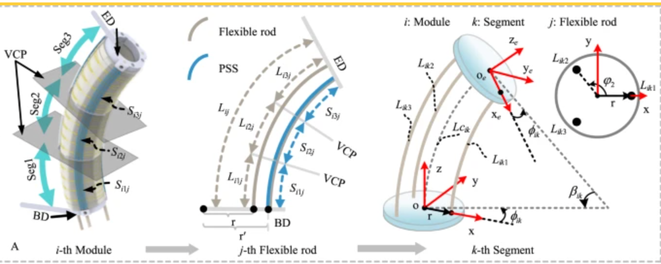
Each segment has id $k$ (k = 1, 2, 3 …), in our current model it is k=2. Each segment $k$ is modelled by three actuation variables. $j$ means the $j$-th actuation length ($j$ = 1, 2, 3). The actuation length is not the same as the stick length. The variables in actuation and configuration space can be expressed as $L_k$ and $Q_k$ respectively.

Actuation Space

actuation space is consist of 3 actuators’ length $l_{k1}$, $l_{k2}$, and $l_{k3}$.

Configuration Space

configuration space for our fix-base robotic arm is $Q_k = (\kappa_k, \phi_k, \beta_k)$ which is the same as the spherical coordinate.
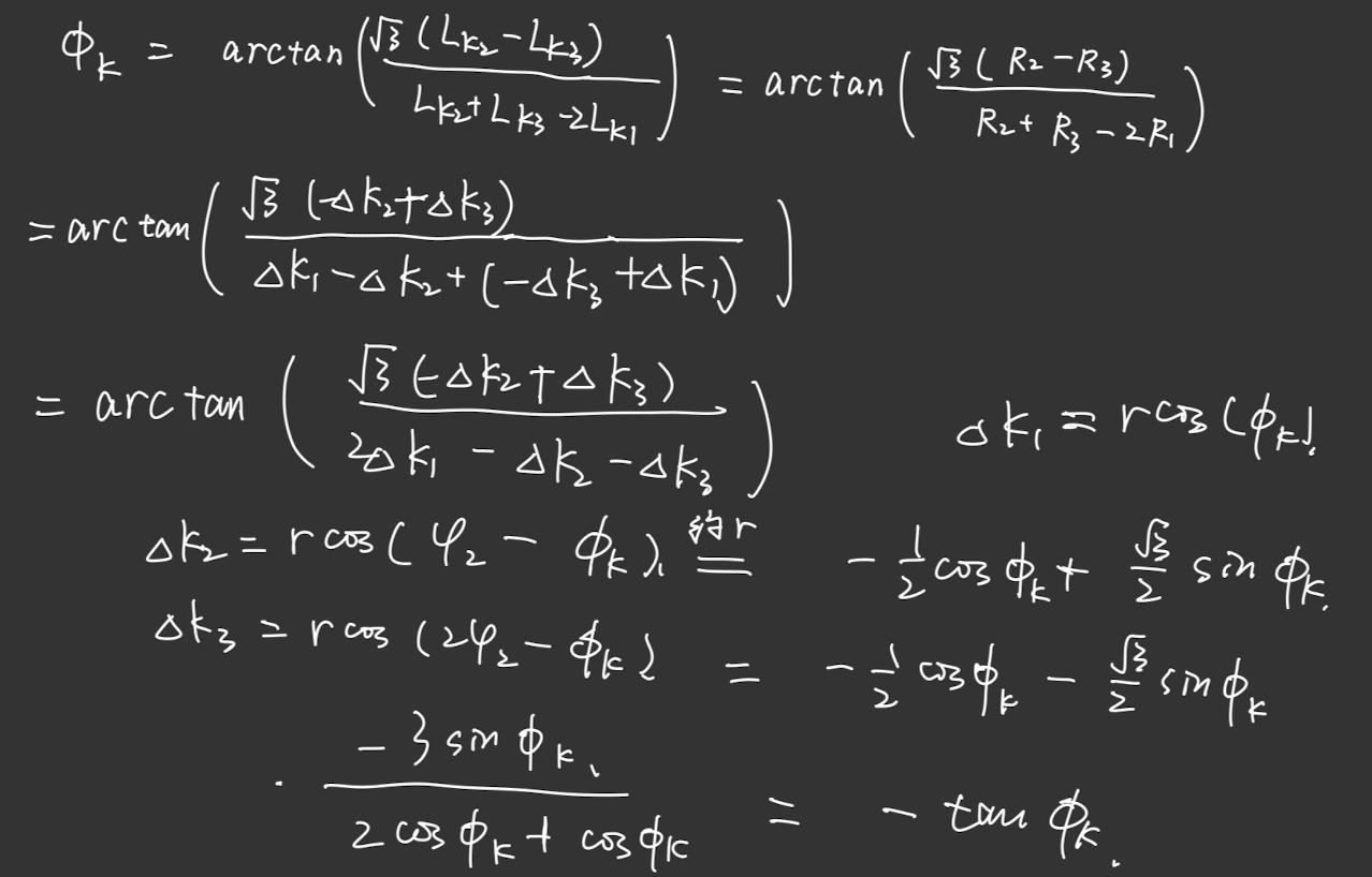
And $\kappa$ denotes the curvature and $\phi$ denotes rotation angle about z-axis.
Or $\kappa$ can be expressed as the arc length $L_{Ck} = \rho_k\cdot \beta_k$, and that $L_{Ck}$ can be expressed as the arm center’s length which is the average of the 3 origamis’ length.
The equations and images are shown below:

1. $L_{Ck} = (L_{C1} + L_{C2} + L_{C3})/3$
2. $L_{kj} = L_{Ck} -\Delta_{kj}\beta_k$ where $\Delta_{kj} = r\cos (\varphi_{kj} - \phi_k)$ and the angles definitions are shown in the figure below.
   
   and $\varphi_{kj} = (j - 1) \cdot 2\pi /3$
3. $\beta_k = \frac{2 \sqrt{L_{k1}^2 + L_{k2}^2 + L_{k3}^2 - L_{k1}L_{k2} - L_{k1}L_{k3} - L_{k2}L_{k3}}}{3r}$
4. $\phi_k = \text{atan2} \left( 3(L_{k2} - L_{k3}), \sqrt{3}(L_{k2} + L_{k3} - 2L_{k1}) \right)$
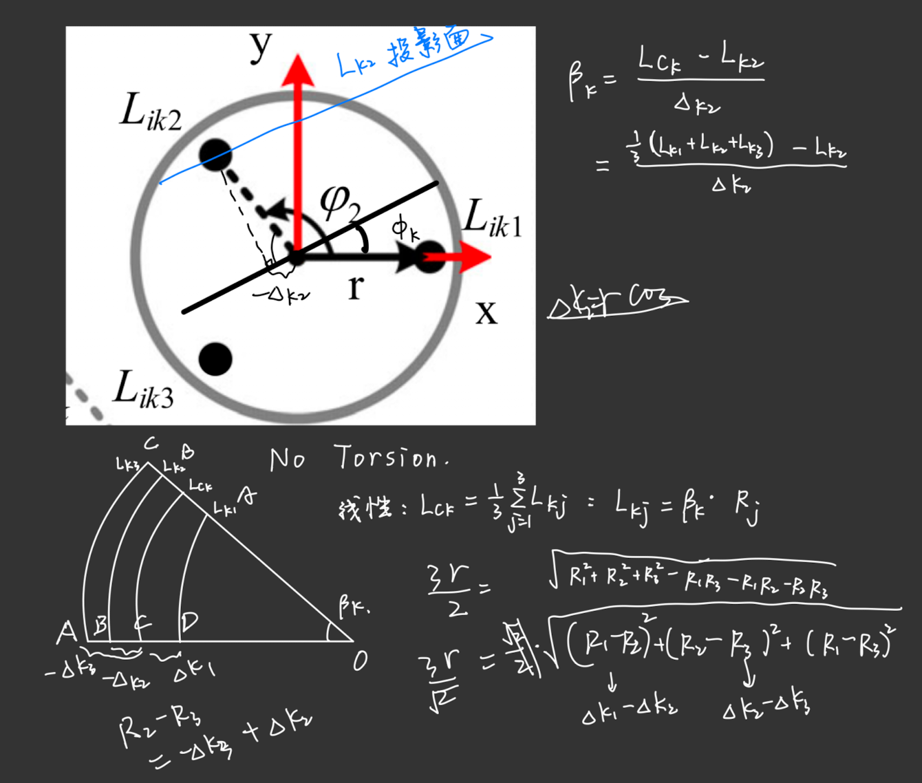
5. $\rho_k = \frac{\beta_k}{L_{Ck}}$, all the equations are shown in the figure below or above
   

Rotations and Positions

the rotation can be expressed as 3 unit rotations about Z axis -> Y axis -> Z axis.
Thus the rotation can be expressed as:

$R_{k}^{k-1}= Rot(Z_{k-1}, \phi_k) Rot(Y_{k-1}, \beta_k) Rot(Z_k, -\phi_k)$

where $k$ is the section id, and the resulting matrix is:

$\begin{bmatrix} \cos\beta_k (\cos\phi_k)^2 + (\sin\phi_k)^2 & (-1 + \cos\beta_k)\cos\phi_k\sin\phi_k & \cos\phi_k\sin\beta_k \\ (-1 + \cos\beta_k)\cos\phi_k\sin\phi_k & (\cos\phi_k)^2 + \cos\beta_k (\sin\phi_k)^2 & \sin\phi_k\sin\beta_k \\ -\cos\phi_k\sin\beta_k & -\sin\beta_k\sin\phi_k & \cos\beta_k \end{bmatrix}$

And then for the position vector it is

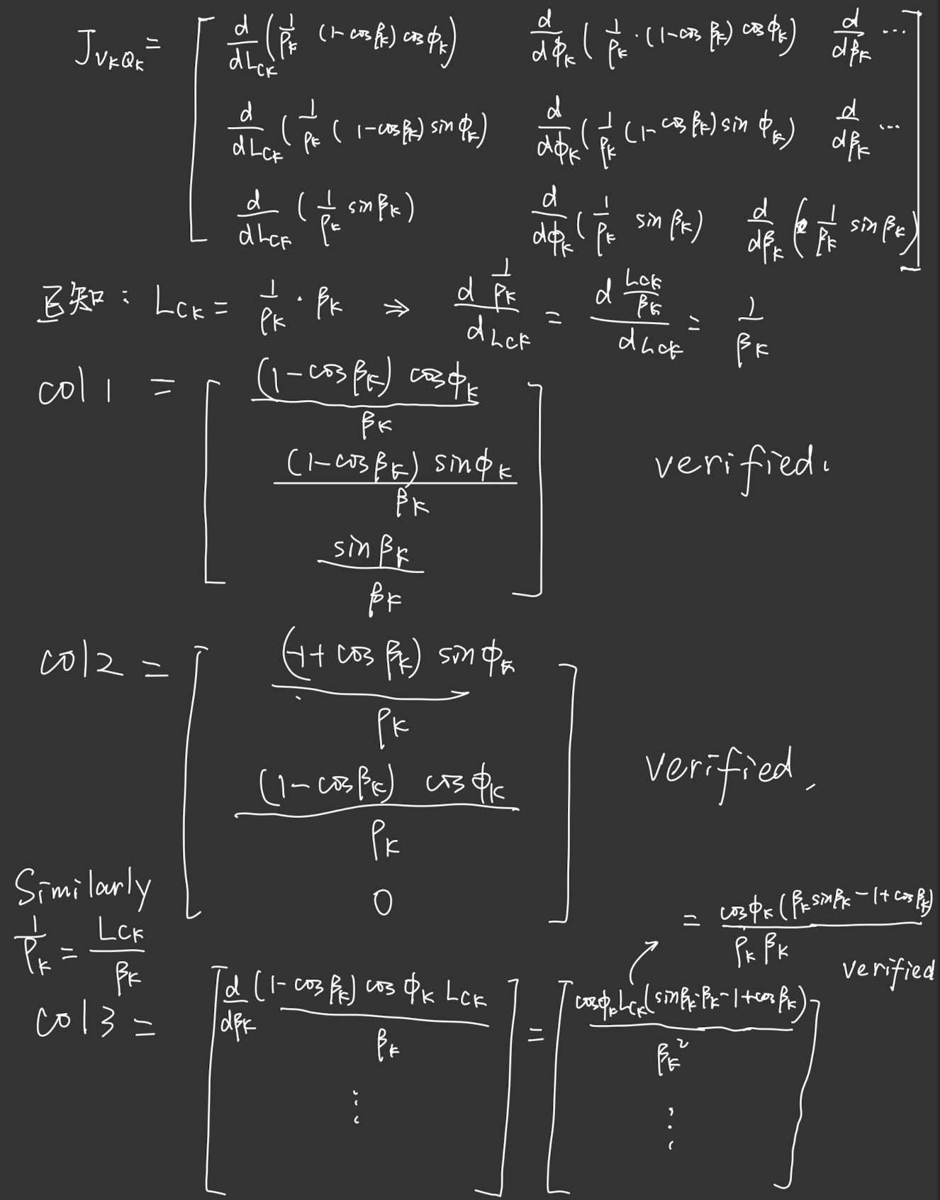
\mathbf{P}_k^{k-1} = \frac{1}{\rho_k} \begin{bmatrix} (1 - \cos\beta_k)\cos\phi_k ,\ (1 - \cos\beta_k)\sin\phi_k ,\ \sin\beta_k \end{bmatrix}^T

And putting them together in 1 transformation matrix is like:

$\mathbf{T}_k^{k-1} = \begin{bmatrix} \mathbf{R}_k^{k-1} & \mathbf{P}_k^{k-1} \\ 0 & 1 \end{bmatrix}_{4 \times 4}$

the above matrix shows the transformation from the k-th arm section to the (k+1)-th arm section, namely we keep right multiply the transformation matrix from the initial base coordinate and get:

$\mathbf{T}_n^0 = \mathbf{T}_1^0 \mathbf{T}_2^1 \cdots \mathbf{T}_n^{n-1} = \begin{bmatrix} \mathbf{R}_n^0 & \mathbf{P}_n^0 \\ 0 & 1 \end{bmatrix}$

Dynamics: Jacobian for Space Transformation

Actuation and Configuration

Since the actuation space can be expressed as the

$\mathbf{J}_{L_k \mathbf{Q}_k} = \begin{bmatrix} 1 & r \beta_k \sin(\phi_k - \phi_{k1}) & -r \cos(\phi_{k1} - \phi_k) \\ 1 & r \beta_k \sin(\phi_k - \phi_{k2}) & -r \cos(\phi_{k2} - \phi_k) \\ 1 & r \beta_k \sin(\phi_k - \phi_{k3}) & -r \cos(\phi_{k3} - \phi_k) \end{bmatrix}$

Then for the multisection’s transformation, we need to map from $\mathbb R^{3k}$ to $\mathbb R^{3k}$, which means that the Jacobian has dimension of $3k\times 3k$. Thus, for stacked sections, it can be expressed as:

$J_{n} = \begin{bmatrix} J_{L_1Q_1} & 0_{3 \times 3} & \cdots & 0_{3 \times 3} \\ J_{L_1Q_1} & J_{L_2 Q_2} & \cdots & 0_{3 \times 3} \\ \vdots & \vdots & \ddots & \vdots \\ J_{L_1Q_1} & J_{L_2 Q_2} & \cdots & J_{L_nQ_n} \end{bmatrix}$

proof

The dynamic equation should be in the form that $\dot q = J_{n} \dot l$ and the higher level $q_i$ should be added with $\sum_{j = 1}^{i-1} J_j \dot l_j$, since the base velocity should be added ahead.

Configuration Space to Task Space

The configuration space and task space are all in 6 dimension: 3 dim for position displacement and 3 dim for angular rotation.
Thus we split the Jacobian into 2 parts:

$J_{X_k} := \begin{bmatrix} J_{v_k Q_k}^T\ J_{\omega_k Q_k}^T\end{bmatrix}^T$

($\begin{bmatrix}A^T\ B^T\end{bmatrix}^T = \begin{bmatrix} A\\ B\end{bmatrix}$) where for single section, $J_{v_k Q_k}$ is $\mathbb{R}^3\to \mathbb{R}^3$

Position Term

The total calculation is from all the 3k origamis’ length to the endpoint’s velocity:

$v_{\text{end}} \leftarrow [\dot \kappa_{1},\dot \phi_{1},\dot \beta_{3}, \cdots\dot \beta_{k}]^T$

which is $J:\mathbb R^{3k}\to \mathbb R^3$.
For a single vector, by differentiate the position vector P with $(\rho =\frac 1\kappa, \phi, \beta)$, and then we could obtain the following:

$J_{v_k, Q_k} = \begin{bmatrix} \frac{1 - \cos \beta_k}{\beta_k} \cos \phi_k & \frac{-1 + \cos \beta_k}{\beta_k} \sin \phi_k & \frac{\cos \phi_k (1 + \cos \beta_k + \beta_k \sin \beta_k)}{\rho_k \beta_k} \\ \frac{1 - \cos \beta_k}{\beta_k} \sin \phi_k & \frac{-1 + \cos \beta_k}{\beta_k} \cos \phi_k & \frac{\sin \phi_k (1 + \cos \beta_k + \beta_k \sin \beta_k)}{\rho_k \beta_k} \\ \frac{\sin \beta_k}{\beta_k} & 0 & \frac{\sin \beta_k + \beta_k \cos \beta_k}{\rho_k \beta_k} \end{bmatrix}$

the detailed derivation is as the following:

And then the recurrence relation can be expressed as the following:

J_{v_k, Q_k} = \begin{array}{c} [ \left (J_{v_{k-1}, Q_{k-1}} - \left (R_k^0 P_k^{k-1}\right)^\wedge J_{\omega_{k-1}, Q_{k-1}}\right ) \ \left( R_k^0 J_{v_k, Q_k}^l \right) \end{array}]

skewed symmetric matrix

Operator $\wedge$ is the skewed symmetric matrix, which turns the vector $v = [v_x\ v_y\ v_z]^T$ into a matrix in the form of

$\mathbf{v}^\wedge = \begin{bmatrix} 0 & -v_z & v_y \\ v_z & 0 & -v_x \\ -v_y & v_x & 0 \end{bmatrix}$

and multiply it with a vector is the same as cross product. Multiplying it with a matrix is the same as doing cross product with each column.

proof

By the dynamic equation, we have relation of velocity:

$v_{P/\mathcal F} = v_{O'/\mathcal F} + ^{\mathcal B}\dot r_{O'P} + \dot\theta\hat k\times \vec r_{O'P}$

namely the new velocity in the new FoR, it adds up the FoR velocity, relative velocity to fixed point and the angular velocity of the new FoR, and also we could write it in the form with no relative velocity (in pure rotation):

$v_P = v_{O'} - \vec r_{O'P}\times \omega$

thus in Jacobian space, we could write as

J_{v_k, Q_k} = \begin{array}{c} [ \left (J_{v_{k-1}, Q_{k-1}} - \left (R_k^0 P_k^{k-1}\right)^\wedge J_{\omega_{k-1}, Q_{k-1}}\right )^T \ \left( R_{k-1}^0 J_{v_k, Q_k}^l \right)^T \end{array}]^T

The $R_k^0 P_k^{k-1}$ is the position vector rotated to the $k-1$-th coordinate and is still the displacement vector $\vec r_{O'P}$
Multiplied by a vector of k sections of configuration space, we could set them to $[\dot q_1, \dot q_2, \dot q_3\cdots \dot q_k]^T$ and the jacobian can be written as $\begin{bmatrix} J_{v_1 Q_1} & J_{v_2 Q_2} & \cdots & J_{v_k Q_k}\end{bmatrix}$ and thus we have the result

$[\sum_{i=1}^k J_{v_i Q_i} \dot q_i]$

which is a $\mathbb R^3$ vector.
Namely the velocity of the end point is the transformed sum of all previous sections’ velocities, which is proven above.

Angular Term

The total calculation is from all the 3k origamis’ length to the endpoint’s angular velocity:

$\omega_{\text{end}} \leftarrow [\dot \kappa_{1},\dot \phi_{1},\dot \beta_{3}, \cdots\dot \beta_{k}]^T$

which is $J:\mathbb R^{3k}\to \mathbb R^3$.
Consider a single section, the Jacobian is simply a coordinate transformation from spherical to world coordinate:

1. $\frac{d}{d\kappa}$: since in the rotational spherical space, the radius of the ball is at constant, thus its 0 in 3 coordinates
2. $\frac{d}{d\phi}$: since for $\phi$ the rotation is about the z-axis, thus the angular velocity is $[-\sin\phi\ \cos\phi\ 0]^T$
3. $\frac{d}{d\beta}$: this is the rotation about the radial direction.
   Then for the stacked sections, the recurse relation is as the following:

$J_{\omega_k Q_k} = [J_{(k-1)\omega_{(k-1)} Q_{(k-1)}}\ \ R_{k-1}^0 J_{\omega_kQ_k}]$

Since the Jacobian needs first be transformed into the (k-1)-th coordinate, it should be multiplied by the rotation matrix first.

proof

multiplied by a vector of k sections of configuration space, we could set them to $[\dot q_1, \dot q_2, \dot q_3\cdots \dot q_k]^T$ and the jacobian can be written as $\begin{bmatrix} J_{\omega_1 Q_1} & J_{\omega_2 Q_2} & \cdots & J_{\omega_k Q_k}\end{bmatrix}$ and thus we have the result

$[\sum_{i=1}^k J_{\omega_i Q_i} \dot q_i]$

which is a $\mathbb R^3$ vector.
Namely the angular velocity of the end point is the sum of all previous sections’ angular velocities, which is easy to prove in dynamics.

Conclusion

The Jacobian from the actuation space to the task space is

$J = [J_{vQ}\ J_{\omega Q}] \times J_{LQ}^{-1}$

Reference

[1] K. Xu and N. Simaan, “Intrinsic Wrench Estimation and Its Performance Index for Multisegment Continuum Robots,” in IEEE Transactions on Robotics, vol. 26, no. 3, pp. 555-561, June 2010, doi: 10.1109/TRO.2010.2046924.
keywords: {Performance analysis;Robot sensing systems;Surgery;Force sensors;Magnetic resonance imaging;Force measurement;Force feedback;Design automation;Spine;Haptic interfaces;Continuum robots;force sensing;haptic feedback;performance index;surgical assistant},
[2]B. Zhao, W. Zhang, Z. Zhang, X. Zhu and K. Xu, “Continuum Manipulator with Redundant Backbones and Constrained Bending Curvature for Continuously Variable Stiffness,” 2018 IEEE/RSJ International Conference on Intelligent Robots and Systems (IROS), Madrid, Spain, 2018, pp. 7492-7499, doi: 10.1109/IROS.2018.8593437. keywords: {Manipulators;Electron tubes;Kinematics;Friction;Tendons;Strips;Lead},
[3]Wang, P., Xie, Z., Xin, W. et al. Sensing expectation enables simultaneous proprioception and contact detection in an intelligent soft continuum robot. Nat Commun 15, 9978 (2024). https://doi.org/10.1038/s41467-024-54327-6
[4]B. A. Jones and I. D. Walker, “Kinematics for multisection continuum robots,” in IEEE Transactions on Robotics, vol. 22, no. 1, pp. 43-55, Feb. 2006, doi: 10.1109/TRO.2005.861458.
keywords: {Robot kinematics;Robot sensing systems;Medical robotics;Manipulators;Hardware;Spine;Shape control;Legged locomotion;Pneumatic actuators;Tendons;Biologically inspired robots;continuum robot;kinematics;tentacle;trunk},